Climb with me beyond the Bell Curve as we unravel the marvels of heavy tails in this exciting journey.
The scientific world would not be what it is today without the normal distribution. It is the foundation of many statistical models for several good reasons. Most importantly, it appears commonly in nature. For instance, if you collect height data from people at your workplace or school and create a histogram, you will likely observe the familiar bell curve. This is because human characteristics, such as weight and height, follow a normal distribution, like many other natural phenomena. One could even go so far as to call the normal distribution nature’s default pattern of randomness.
But this is only the tip of the iceberg. For example, roll a die many times and count the average number of times you rolled a six. In the beginning, your results might appear quite chaotic - three sixes in a row and then none for a long time… However, as you continue rolling, a familiar pattern emerges; the distribution of the average starts to resemble a normal distribution. This phenomenon turns out to be quite universal as the shape of the original data typically does not matter; if you add up enough of it, the result starts looking like a normal distribution.
This principle is known as Central Limit Theorem (CLT) and it is responsible for the widespread use of normal distributions in many models. So, is this it? Is the normal distribution all you need to remember from your statistics course? Definitely not! What is more, things can go terribly wrong when we assume that something is normal, when it is not. Let me show you that this is true with one simple example.
You have probably heard about the financial crisis in 2008. Up until that point, pricing and risk models in finance, such as the Black-Scholes model, relied heavily on the assumption of a normal distribution. However, this assumption was more often than not violated in practice. In consequence, the models were underestimating the risk of extreme or rare events which is commonly called the tail risk.
This means that people and financial institutions did not fully realize how bad things could get if an extreme event happened, and therefore were not prepared or insured against it. Although the 2008 crisis was years in the making and already in 2006 we could observe its first effects on the U.S. housing market, it is the fall of Wall Street bank Lehman Brothers in September 2008, the largest bankruptcy in U.S. history, that tipped the scales.
Chaos ensued as everyone abruptly began losing huge amounts of money, leading to a worldwide financial crisis.
While the causes of the crisis were numerous and complex, it is the underestimation of tail risk and improper risk management that can be considered the primary culprits. So, how do we properly account for the tail risk? Heavy tails can help with this! Whether this is a totally new territory for you or if you are already versed in heavy tails but seeking an engaging read, join me on this journey where we (re)discover heavy tails and some of their magical properties and applications.
What are heavy-tails?
Heavy tails, or more precisely heavy-tailed distributions, represent a type of data where the likelihood of extreme events is greater compared to more common distributions, such as the normal or the exponential distribution. They are used to describe situations where rare or unusual things occur more often than you would think. For example, earthquake magnitudes are heavy-tailed. This means that small earthquakes occur frequently, almost continuously and typically we do not even notice them. But, once in a while, an extreme earthquake happens, like the Japan earthquake in 2011 or the Indian Ocean earthquake in 2004. Prediction models based on normal distribution would deem an earthquake on such scale as almost impossible, while two of them already happened in this century, causing hundreds of thousands of casualties. This shows that heavy tails are crucial to properly understand and model the risk of extreme earthquakes.
The name heavy tail comes from a visual representation of the distributions (see Figure 1 below). Here we compare the right tails of an exponential, normal, and Pareto distribution — the most famous example of a heavy-tailed distribution. The line corresponding to the Pareto distribution is highest for large indicating that the probability of a very large data point or event is higher than for the other two distributions.
Figure 1: Tail comparison of Pareto, Normal and Exponential distribution.
Heavy tails may seem mysterious simply because they are less known. In the early evolution of probability theory, the focus primarily rested on the elegance of normal distributions and their widespread applicability. It wasn’t until the 20th century that scientists like Vilfredo Pareto and Paul Lévy began advocating the existence of distributions with heavier tails. However, this was not enough to convince the scientific world to depart from the comforts of the normal distribution and venture towards the unknown heavy tails.
For many years, heavy-tailed theory was studied only by a few and considered more as a mathematical curiosity rather than a tool that is useful in practice. People simply were not convinced that such a high likelihood of extreme events could be true in real life. However, nature has mysterious ways of surprising us and this holds true for heavy tails as well. With increasing digitization, we became more and more capable of collecting and analyzing data and suddenly we realized that there is an entire world of heavy tails beyond the "bell curve" and that examples of heavy tails are found all around us. To name a few, the following can be heavy-tailed:
Natural disasters such as magnitudes of earthquake distributions;
City sizes;
Packet sizes in Internet traffic;
Insurance claim sizes;
Number of connections in real-world networks;
Sizes of disease outbreaks.
With these new findings, we began adapting our mathematical models to reflect the possibility of rare events that many of the classical approaches ignored. Unfortunately, this revolution has been primarily driven by catastrophic events like the financial crisis, but better late than never!
Unorthodox properties of heavy-tails
Another reason why, for a long time, people did not believe in the occurrence of heavy tails in practice is their somewhat unorthodox properties. For example, a heavy-tailed distribution can have an infinite variance, or even an infinite mean. This is problematic for a couple of reasons. First, the classical statistics revolve around averages and variances. We use them to describe and compare data in a meaningful way, perform hypothesis testing, etc. However, if the mean or the variance is infinite, none of these methods can be applied. Second, imagine that some natural phenomenon has an infinite mean; think for example of earthquake distributions. If you collect a sample, no matter how large, you will be able to compute its average value and it will always be finite. This is a bit counterintuitive and makes the estimation of heavy-tailed phenomena less straightforward than that of light-tailed (not heavy-tailed) phenomena.
What about the Central Limit Theorem that “magically” transforms distributions into a normal distribution? Can we use it to make some sense out of the heavy-tailed distributions? Yes! … and no. CLT requires the variance to be finite, and, as we know by now, not all heavy tails have that. However, it does not mean that there is no regularity to these heavy-tailed distributions. Instead of being transformed into a normal distribution, they can be transformed to another heavy-tailed distribution with infinite variance.
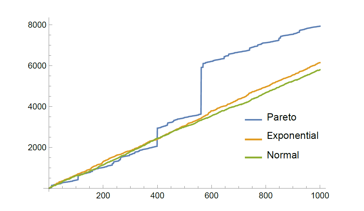
Yet another non-conforming feature of heavy tails becomes evident when examining Figure 2. There, we took a sample of 1000 data points and for each value on the -axis, we plotted the sum of the first data points in our set. Mathematically, we would call this object a random walk, which is an extremely useful model for analyzing time-dependent processes such as the movement of particles or stock market prices.
Figure 2: Different behavior of random walks with heavy- and light-tailed increments.
Looking back at the graph, if the samples come from any light-tailed distributions, we could approximate the plot with a straight line. However, for the Pareto case (which is a heavy-tailed distribution), we observe visible jumps, caused by extreme events. In this case, a straight-line approximation no longer seems like a good idea. It seems that some distributions just do not want to conform and there is nothing more we can do other than accept them as they are. But that is alright, because, as it turns out, some of their properties are intuitive, well-understood, and can make analysis quite simple.
Conspiracy vs. Catastrophe Principle
A well-known and intuitive characteristic principle of heavy tails is the catastrophe principle. Let me explain it using an example. If the total wealth of people in a train is a few million dollars, then most likely you are traveling with one millionaire and the rest of the passengers have an average wealth. This is because wealth distribution is typically heavy-tailed. This example can be generalized to a catastrophe principle, which tells us that if a sum of heavy-tailed data points is large, it is most likely due to one data point being extremely large, a.k.a a catastrophe.
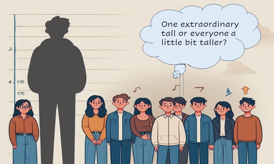
Now, imagine that you travel in a train and the average height of the passengers is more than two meters. Does that mean that you are traveling with a 10-meter-tall giant? Probably not! It is more likely that you travel with a basketball team where all players are exceptionally tall. This is an example of a conspiracy principle, as all data points in your height sample “conspired” by having an above-average height. Height distribution is light-tailed because extremely tall people do not occur due to biological constraints. This is why the conspiracy principle applies in this case. These two examples illustrate fundamental differences in the behavior of heavy-tailed distributions, as opposed to the light-tailed distributions we are more familiar with.
The intuition that comes from the catastrophe principle is extremely useful when analyzing processes related to heavy tails and especially their extrema. For example, imagine a supermarket queue where the number of items each customer buys is heavy-tailed. We are interested in the probability of a very large waiting time. Although infinitely many different scenarios could lead to this, we only need to care about one! Most likely the large waiting time is caused by only one extreme event, for example, a customer who decided to stock up for the entire year. This is where the beauty of heavy tails lies: using the catastrophe principle we can bring down a complex problem to the analysis of a single instance that is tractable. But there is so much more.
Over the years, this idea has been polished and perfected, resulting in theorems for heavy-tailed processes which allow us to understand more and more complex heavy-tailed problems. The recently published mathematics book The Fundamentals of Heavy Tails provides a comprehensive account of properties, emergence, and estimation of heavy-tails. This book can help you navigate through the world of heavy tails and reveal other properties that could not be covered in this text.
To sum up, through this blog, I aim to show that there is more to statistics than the familiar bell curve and other light-tailed distributions. Heavy tails are prevalent, and they adhere to non-standard yet intuitive principles. What is more, things can go very wrong when we ignore tail behavior. So, the next time you stumble upon heavy tails, do not ignore them; embrace them. Despite appearances, they turned out to be quite tamable.
In 2014, in the Netherlands, Belgium and Germany, the average person spend approximately 40 hours in a traffic jam - that is 5 work days! In this article, I will explain how mathematical models with uncertainty help traffic engineers to make decisions that improve traffic.
Despite our level of development, the pandemic has been continuously causing us struggles for two years. This gives rise to an obvious question: How can contemporary science not deal with a flu-like virus?
Mathematician Bert Zwart of the Dutch National Research Institute for Mathematics and Computer Science (CWI) and his colleagues, Tomasso Nesti (CWI) and Fiona Sloothaak (Eindhoven University of Technology) have now proposed a new explanation on how large electric power blackouts can occur.
Have you ever wondered what makes a video go viral? Or how it is possible that they can spread so quickly? Maybe you didn't (that's fine), but many economists, marketeers, and even mathematicians have wondered.
In this article, we will discuss a mathematical riddle that "seems impossible even if you know the answer". It is better known as the 100 prisoners problem.

 heavy tail
 comes from a visual representation of the distributions (see Figure 1 below). Here we compare the right tails of an exponential, normal, and Pareto distribution — the most famous example of a heavy-tailed distribution. The line corresponding to the Pareto distribution is highest for large
  indicating that the probability of a very large data point or event is higher than for the other two distributions.
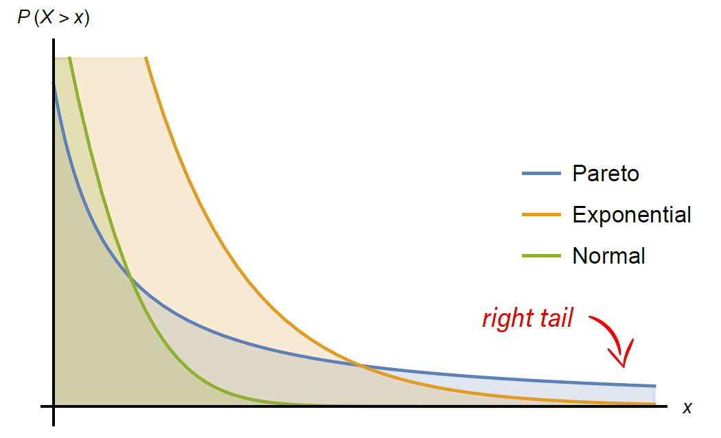
 on the