Chemical reactions evolve in the same way as water flows through a network of rivers. When describing a chemical reaction you can imagine that the concentrations of the reactants are flowing through the reaction network in the same way as water flows through the network of rivers. Kinetic models describe how the concentrations flow through the states of the molecular species in the network.
In the preceding article we discussed how one can construct a reaction network describing the reactions occurring in a chemical system. Reaction networks are a useful tool when we want to describe complex reaction mechanisms. Such reaction mechanisms often involve numerous intermediate and product molecular species. The molecular graph of a reactant is gradually transformed into the graph of a product by following some predefined reaction steps. The reaction network allows experts to explore various reaction pathways in great detail. In this article we will focus on how to reconstruct a kinetic model from the reaction network.
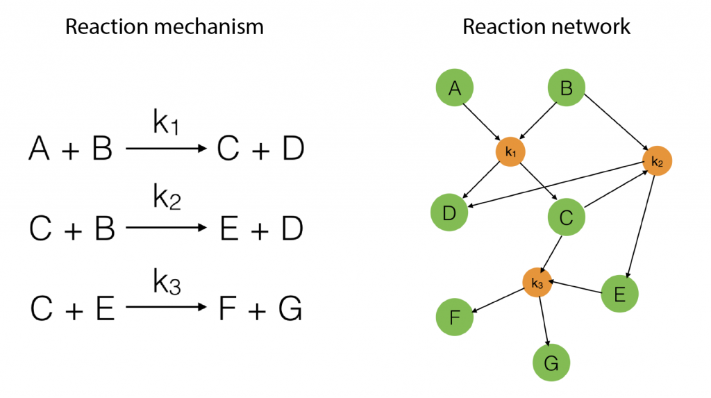
To start with, suppose we have a reaction mechanism that involves several steps and consider the corresponding reaction network. Such a mechanism is illustrated in Figure 1 below.
Figure 1: An example of a simple reaction mechanism
Kinetic Model
A kinetic model is a system of ordinary differential equations that describes how the concentrations of molecular species taking part in the reaction mechanism are changing in time. The equations in the kinetic model are constructed in terms of reaction rates. Intuitively, the reaction rate describes how often the reaction happens and which molecular species are the reactants. Reaction rates depend in general on the concentration of the reactant species and on the conditions in which the reaction happens (temperature, pressure, volume).
With no doubles, the kinetic model is the central idea in the studies of co-occurring chemical reactions, it is basically a dynamical system that tells us how the concentrations of chemical species evolve in time. This dynamical system may involve many equations, but it is typically very ‘sparse': only few variables per one equation. Chemists like represent this sparse structure by a network. The properties of the dynamical system can then be mapped to the topological peculiarities of this reaction network.
says dr. Ivan Kryven, from the van 't Hoff Institute for Molecular Sciences, University of Amsterdam.
Lets see an example, suppose we have two reactants, denoted by and that molecules of react with molecules of to yield the two products . Schematically this is depicted as follows:
Then the rate of this reaction is
where is some coefficient. In this equation, are the concentrations of the corresponding molecular species and their product determines the probability that they find each other and react. The higher the concentrations, the easier for the molecules to collide. The exponents specify how many molecules of each reactant are needed for the reaction to happen. The example above requires molecules of and molecules of . The value of gives an overall order of a reaction: the total number of reactant molecules. The most common reactions are of the first and the second order: they happen with one or two molecules. The first or the second order reactions are also called unimolecular or bimolecular, respectively. The coefficient , called the rate coefficient, includes the information about the conditions in which reaction happens (temperature, pressure, etc). Rate coefficients are usually obtained from the experiments or from quantum chemical calculations, these details are omitted from the article and we suppose that the values of are known for the considered reactions.
The main motivating question leading to kinetic models rises. How do the concentrations of the various molecular species change given the rates of the reactions? Suppose we have a reaction mechanism where molecular species take part. Then we would like to know what the concentration of each one of them is at a given time , these concentrations will be denoted by . The left hand side of each equation in the kinetic model is the partial derivative of a concentration of a particular molecular species with respect to time, , . This describes the speed at which the concentrations change in time. On the right hand side we relate the changes in the concentrations to the rates of the various reactions. This leads to equations of the following form:
In order to understand these equations we note that, when measuring the concentration of a given molecular species during a chemical reaction, there are reactions that will increase its concentration (produce this species) and reactions that will decrease its concentration (consume this species).
The positive contributions come from rates of reactions that include as a product (the reactions that produce this species). The negative term includes all the rates of reactions where the plays a role of a reactant (it undergoes a transformation and its concentration decreases)!
Usually kinetic models are constructed manually. The problem comes when the reaction mechanism is too big and constructing a kinetic model requires a lot of effort and attention. Then, the question is: how to transform the information from the reaction network to the kinetic model?
The reaction network can be described by the adjacency matrix of size , where . Here represents the number of molecular species and the number of reactions. has two types of nodes, nodes corresponding to:
molecular species
and reactions.
Nodes corresponding to molecular species have a weight corresponding to their initial concentration, denoted by . The weight of a node corresponding to a reaction denotes the rate coefficient of the corresponding reaction.
The rate equation for each state of the molecule is reconstructed by exploring its neighborhood in the reaction network. The incoming edges denote the reaction pathways that contribute to the concentration of the species considered while the outgoing edges denote the reaction pathways that lead to a decrease in the concentration of the species considered.
In what follows we are going to describe the formal transition from the reaction network to the reaction rate equations. We will only consider reactions of first and second order, and their mixtures, as most of the reaction mechanisms involve mixtures of the first and second order reactions. For this purpose, we will use three main components:
- adjacency matrix of the reaction network,
- vector of concentrations of each molecular species and
- vector of rate coefficients for each reaction from the reaction network.
The entries of that correspond to the reaction nodes in the adjacency matrix and the entries of that correspond to the species nodes in the adjacency matrix are zero. The shape of all these quantities is illustrated in Figure 2 below.
Figure 2: An adjacency matrix, concentration vector and coefficient vector of a simple second order reaction networks introduced in Figure 1
First order reactions
We consider first the case of a reaction mechanism that consists of only first order reactions. For a state node , the differential equation describing the distribution of species concentration is written in terms of the adjacency matrix of the reaction network and coefficient vector ,
The difference determines the sign of the term: a positive sign means that the concentration of the molecular species increases, a negative sign that it decreases! The equation in \eqref{eqn:secondform1} conveys exactly the same information as equation \eqref{eqn:concentrations}, it is just written in terms of the reaction network!
Second order reactions
The differential equation given above for can be extended to cover reactions of the second order, then it takes the form
The product sign in the last part of the equation accounts for the number of reactants in the reaction.
Exercise: Write the equations in \eqref{eqn:secondorder} explicitly for the reaction described in Figure 1 (use the matrix representation in Figure 2). Interpret these equations!
For this reaction we have (that is three reactions, ) and (that is seven species taking part in the reaction). Hence for the first species, denoted by , we have
To understand what these equations mean lets see at the first equation for . Molecules of type only react with to give molecules of types . Hence the concentration of can only decrease, that is why the minus sign appears. And this will keep going until there are no molecules of type or left. The higher their concentration the faster they will react with each other, that is why the product appears.
Mix of first and second order reactions
Let us split the vector of rate coefficients , where is non-zero for first order reactions and is non-zero for second order reactions.
A combination of equations \eqref{eqn:secondform1} and \eqref{eqn:secondorder}, together with the corresponding rate vectors yields the differential equation for a mixed reaction network,
We can solve the system of equations in \eqref{eq:mixed} numerically, this provides us the information about the distribution of the concentrations of all species present in the resulting reaction network. In the end, one might be interested in tracking the cumulative amount of concentration of various functional groups rather than specific molecular structures. This can be done by lumping the concentrations of all the species according to the functional groups they contain. As it was discussed in the preceding article, functional groups are defined as patterns on molecules. By doing so, one can observe the global picture of the chemical process and compare the results to the experimental data, that are usually reported in terms of distributions of various functional groups.
To summarize, in this article we have introduced the systematic way of reconstructing the reaction network into the kinetic model of the chemical process. The kinetic model describes how the concentrations of molecular species travel in time from one state of the reaction network to another. Solving the kinetic model allows to validate the result by comparing the distribution of various functional groups in time with the kinetic data from the experiments. This way of dealing with the complex chemical systems is quite generic and allows to explore them in a great detail.
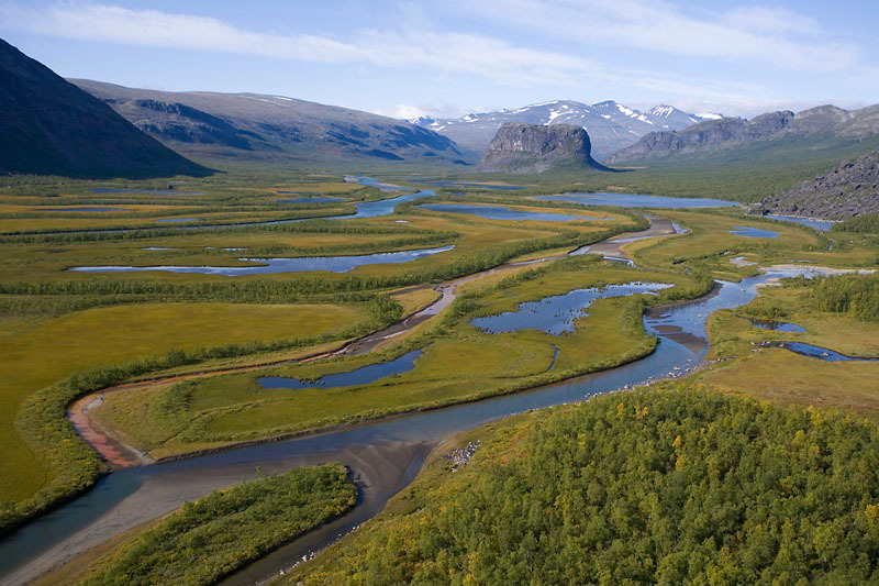
In 1995, a flood in the town of Itteren led to the evacuation of 250 000 people and a million animals. Consequently, the Dutch regional water authorities were tasked with calculating how often an area overflows, such that better measures could be taken. How do these calculations work?
Getting to class on time isn't hard, if you leave on time and know the fastest route. But what’s the fastest route when the hallways are crowded? For their final high school project, Dylan and Tobias worked on finding the most efficient ways to navigate school during peak hours.
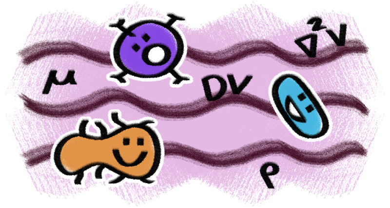
The gut microbiome works hard to keep you healthy. To understand it, we need to know how nutrients travel through the gut. This is where gut flow enters the story. How can we simulate gut flow with mathematics?
We want our guts to be filled with a diverse range of mutually beneficial and competitive interactions, a perfect blend of friends, frenemies, and enemies to keep our guts active and body on its toes. Read how networks can help understand these interactions!
 and that
  molecules of
  react with
  molecules of
  to yield the two products
  . Schematically this is depicted as follows:
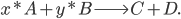
![Rate = k*[A]^x*[B]^y,](https://www.networkpages.nl/wp-content/plugins/latex/cache/tex_a662c31683bfebe73e9609c673fb0d2d.gif)
 is some coefficient. In this equation,
 ![[A], [B]](https://www.networkpages.nl/wp-content/plugins/latex/cache/tex_03447f154f66f43e99444bfe4717ea76.gif) are the concentrations of the corresponding molecular species and their product determines the probability that they find each other and react. The higher the concentrations, the easier for the molecules to collide. The exponents
are the concentrations of the corresponding molecular species and their product determines the probability that they find each other and react. The higher the concentrations, the easier for the molecules to collide. The exponents  specify how many molecules of each reactant are needed for the reaction to happen. The example above requires
  gives an overall order of a reaction: the total number of reactant molecules. The most common reactions are of the first and the second order: they happen with one or two molecules. The first or the second order reactions are also called unimolecular or bimolecular, respectively. The coefficient
  molecular species take part. Then we would like to know what the concentration of each one of them is at a given time
  , these concentrations will be denoted by
  . The left hand side of each equation in the kinetic model is the partial derivative of a concentration of a particular molecular species with respect to time,
  ,
,  . This describes the speed at which the concentrations change in time. On the right hand side we relate the changes in the concentrations to the rates of the various reactions. This leads to equations of the following form:
 come from rates of reactions that include
  as a product (the reactions that produce this species). The negative term includes all the rates of reactions
  where the
  , where
  . Here
  the number of reactions.
  . The weight of a node corresponding to a reaction denotes the rate coefficient
  - adjacency matrix of the reaction network,
 - vector of concentrations of each molecular species and
 - vector of rate coefficients for each reaction from the reaction network.
 that correspond to the reaction nodes in the adjacency matrix and the entries of
  that correspond to the species nodes in the adjacency matrix are zero. The shape of all these quantities is illustrated in Figure 2 below.
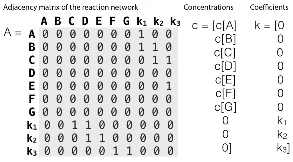
 , the differential equation describing the distribution of species concentration
  is written in terms of the adjacency matrix of the reaction network
  determines the sign of the term: a positive sign means that the concentration of the molecular species increases, a negative sign that it decreases! The equation in \eqref{eqn:secondform1} conveys exactly the same information as equation \eqref{eqn:concentrations}, it is just written in terms of the reaction network!


 , where
  is non-zero for first order reactions and
  is non-zero for second order reactions.
 yields the differential equation for a mixed reaction network,