It is some time now I wanted to write about a mathematical result I think is really beautiful. It comes from percolation theory and in this article my goal is to describe it and show why I find it so beautiful.
Percolation Theory
Percolation theory is a branch of mathematics at the interface between probability theory and graph theory. The term 'percolation' originates from materials science. A representative question (and the source of the name, from Latin percolare, "to filter" or "drip through") is as follows. Suppose some liquid is poured over a porous material. Will the liquid be able to make its way from hole to hole and reach the bottom? To gain insight into how we might answer this physics question, we study a mathematical model. We model this phenomenon using a three-dimensional network of nodes in which the edges between any two neighbors can be open with probability (allowing the fluid to pass), or closed with probability . In this model, one would like to know how likely it is that an open path (that is, a path, each of which has an "open" connection) from top to bottom.
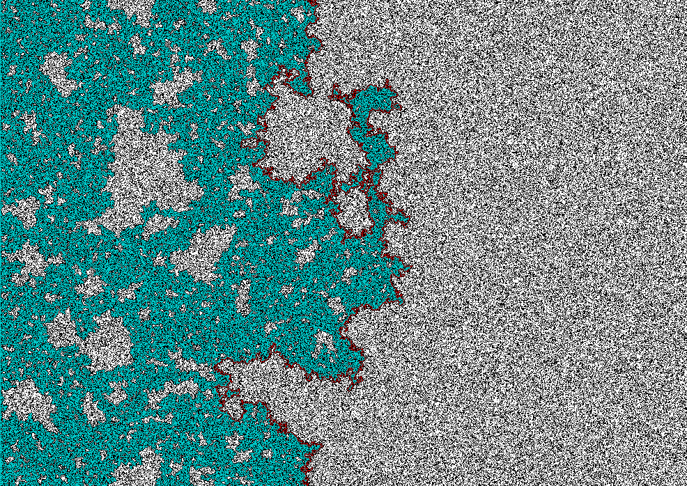
In the animation below, developed by Martijn Gösgens from the Tu Eindhoven, you can see yourself how percolation on a grid works. You can choose the probability of an edge being open, and if you click on Percolate then you obtain a network where some edges are removed. The nodes in green are those from which the bottom can be reached via an open path. An open path from the top layer to the bottom layer, if present, is shown in red.
In mathematics, percolation is considered the process of randomly removing edges in a network. In the model above, percolation thus corresponds to keeping the edges open or closed between the buttons. Let's see what percolation would mean in some other examples of networks.
Networks
Many everyday phenomena can be described by networks. Take, for example, congestion at the national highways. The road network describes the possible routes that cars can take and indicates the maximum traffic flow that can be processed. An electricity power network describes how electric current can flow. A social network describes who comes into contact with whom, whereby a contact can have different interpretations, such as real friends who have physical contact, followers on Twitter, or people who keep in touch on an online platform.
In such networks, connections may be affected by external factors, and may be lost or disabled. In a road network, for example, roads can be blocked by an accident, in an electricity network connections can be switched off due to overload, thunderstorms, or accidents. In a social network, people can transfer gossip, information, but also a virus to their acquaintances. These are all examples of random events on a network's connections. Such random events at the connections of a network are often studied mathematically by means of models from percolation theory.
In percolation theory people are interested in the properties of the network after percolation, i.e. the random removal of a number of connections. In a power network, for example, it is very important to know how electricity will be distributed over the other connections if any number of connections are down. In a social network of contacts, people often want to know how quickly, and to what extent, information, or a virus, will be spread to other people through their acquaintances.
And the math?
Let's look at a mathematical example of percolation on a network. As explained earlier, a network consists of objects that are interconnected. Mathematicians call such a network a graph, the objects are nodes, and the connections are edges. For example, take the graph in Figure 1. This graph contains 18 nodes and 33 edges.
Figure 1: A graph with 18 nodes and 33 edges.
Now we are going to do the following experiment: For each edge we are going to throw a fair coin, if heads comes out the edge will remain in the graph, but if tails comes out we will remove this edge. So if we're going to do this for each edge, this means that if we toss a coin 33 times, we'll most likely get a new graph with some edges removed. In percolation theory one is interested in the structure and properties of the graph that remains after percolation. In Figure 2 we see an outcome of percolation on the graph in Figure 1.
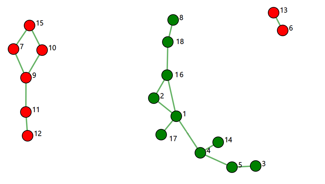
Figure 2: The graph after percolation
The math can say a lot more than what we see in this picture. The number of edges that will be removed is generally a random variable that we can describe mathematically by means of a binomial distribution with parameters and .
So, using the properties of the binomial distribution, we see that the expected number of edges that will be removed after percolation is , so about half of the edges. This makes sense since every edge is removed with probability 0.5. In Figure 2 we see that 16 edges were removed. If we repeat this experiment several times, we will notice that sometimes more or fewer edges will be removed. This deviation from the expected number of removed edges is described by the variance, which for a binomial distribution is equal to , so in this example.
You can also think of more complicated questions: for example, how likely is it that the graph will remain connected after percolation? Or how large are the connected components in the graph if it is not connected? A graph is said to be connected if there is a path from one point to another between any two nodes in the graph. For example, the graph in Figure 2 is not connected, but contains three connected components, the largest of which is shown in green. Such questions are central to percolation theory and require rigorous and technical mathematical analysis to answer them. For the interested reader, later we will briefly explain how connectivity can be studied mathematically. But first, we're going to talk about a concept that scientists are fascinated with, that of a phase transition!
Jumping between phases
A very interesting phenomenon in percolation theory is that of a phase transition. The term originates from thermodynamics and refers to the situation a system exhibits a transition from one state to another when some parameter reaches a critical value. Think for example of water becoming liquid from ice when the temperature raises to 0 degrees Celcius. In the follow up we discuss two more examples of a phase transition, one from everyday life and one mathematical, the beautiful result I mentioned in the beginning. Let's start with the mathematical example.
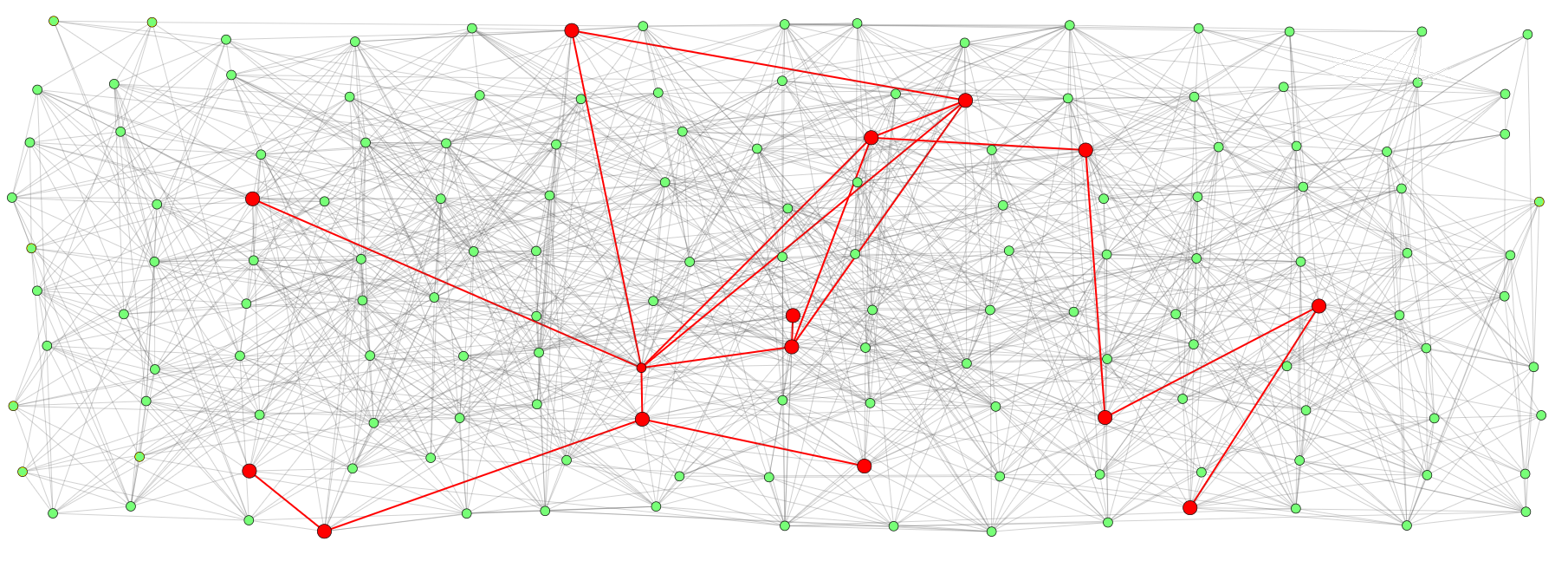
Take nodes and connect all pairs of knots together with one edge. The resulting graph is called in mathematics the complete graph on nodes. For percolation on the complete graph at nodes we are going to keep each side with probability . If then all edges will definitely be conserved, if then about half of all edges will be removed, and if then all edges will be definitely removed.
Now let vary between 0 and 1 and see what the resulting graph will look like after percolation. Think of this as a movie where represents time and the image on your screen is the graph after percolation with probability . So in the beginning, for , you see an empty graph because all edges are removed. As grows, fewer and fewer edges are removed.
All five graphs have 200 nodes. The value for p differs, from left to right it is equal to 0.002, 0.004, 0.006, 0.008 and 0.01.
Two mathematicians, Paul Erdős and Alfred Rényi, proved in 1960 that when is roughly equal to , and is large enough, something interesting happens with the graph: there is a phase transition! This means that for , with , the graph with a high probability is not connected after percolation, but for values of , with , the graph with a high probability is connected! So there is a transition from one phase (not connected) to another phase (connected). The value , for large enough , is in this case a sharp boundary for connectivity in the complete graph.
This a famous result from percolation theory and, although I know about it since a long time ago, I only understood why the logarithm comes into play some time ago when I read the detailed proof. For those of you who want to have a look at a sketch of the proof of this result have a look at the additional part below. Otherwise feel free to proceed to the second example!
We take the probability equal to , and we outline the proof that if then the complete graph after percolation, where we start to keep sides with probability , remains connected with high probability. What is amazing in the proof is that in order to prove that the graph after percolation is connected, it is sufficient to prove that after percolation no isolated nodes are formed! A node is called an isolated node if it is not connected to any of the other nodes. In [Remco van der Hofstad, Random Graphs and Complex Networks, Volume 1, Section 5.3] it is proved that
where represents the number of isolated nodes in the graph after percolation. So this is a random variable and we can write it as a sum of indicator functions as follows
The indicator function of an event is equal to 1 if event happens, and equal to 0 if does not happen. We also use the notation to describe the probability of an event, after percolation with probability .
The result in (1) is wonderful because it is not at all obvious why the fact that no isolated points arise after percolation implies connectivity of the graph. For example, two or more disjoint components could exist. But it turns out that, for big enough, such an event is very rare. Given (1) it is thus sufficient to show that, as , and for (depending on ) such that ,
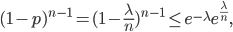
Thus, we need to determine the expected number of isolated nodes after percolation, i.e. . A node is isolated if it is not connected to another node. During percolation we are going to remove edges with probability . So this means that a node is isolated after percolation if all edges with the other nodes in the graph are removed, this happens with probability
where the inequality follows from . Using this result, and because the expectation of a sum is equal to the sum of the expectations, we see that for the expectation in (2) it holds that
From (2) it follows that
as . So we see that the case , or , is a sharp boundary for connectivity in the complete graph! Moreover, we also notice that for greater than the boundary value of , all nodes belong to one component, which is called the “giant component”. To learn even more about the math behind networking and percolation theory, check out our online mathematics class on networks.
And suddenly everyone knows a gossip
The second example of a phase transition comes from everyday life and will sound familiar to many of you. Think of a social network. Social networks are the basis for exchanging information, spreading news and gossip. Depending on the structure of the social network of contacts, but also on the likelihood of information being exchanged with a contact, it may happen that a gossip is only spread locally, it may not be spread at all, but it may also happen that it becomes viral. goes and that everyone in the network knows the gossip. When disseminating information, there is therefore also a phase transition!
Figure 3: A gossip may spread only locally if the probability is too low
How can we use what we have learned to better understand the dissemination of information? Let us assume that our contact network is in fact the complete graph, ie all nodes can communicate with all other nodes. Now imagine that at some point in our model node comes to know some very catchy gossip. In the next time step, there is a probability that the gossip is told to a neighbor node . We can think of this as the outcome of flipping an unfair coin, which with probability lands on “heads”. Now it doesn't matter whether we toss this coin at the beginning of the model to decide whether the gossip is passed from to when finds out about the gossip, or whether we do this as soon as actually finds out about the gossip.
If we continue to reason like this, we can flip a coin for every pair of knots, and add only the edges for which we get “heads” to the network. These are exactly the edges where the gossip is passed if one of the adjacent nodes finds out about the gossip. But this looks exactly like percolation on a complete graph where each edge is likely to be preserved with probability ! In the long run, the gossip will spread throughout the entire components containing the first source nodes. When is so large that , there is a good chance that the first source nodes are in the giant component, with the result that everyone gets to know the gossip!
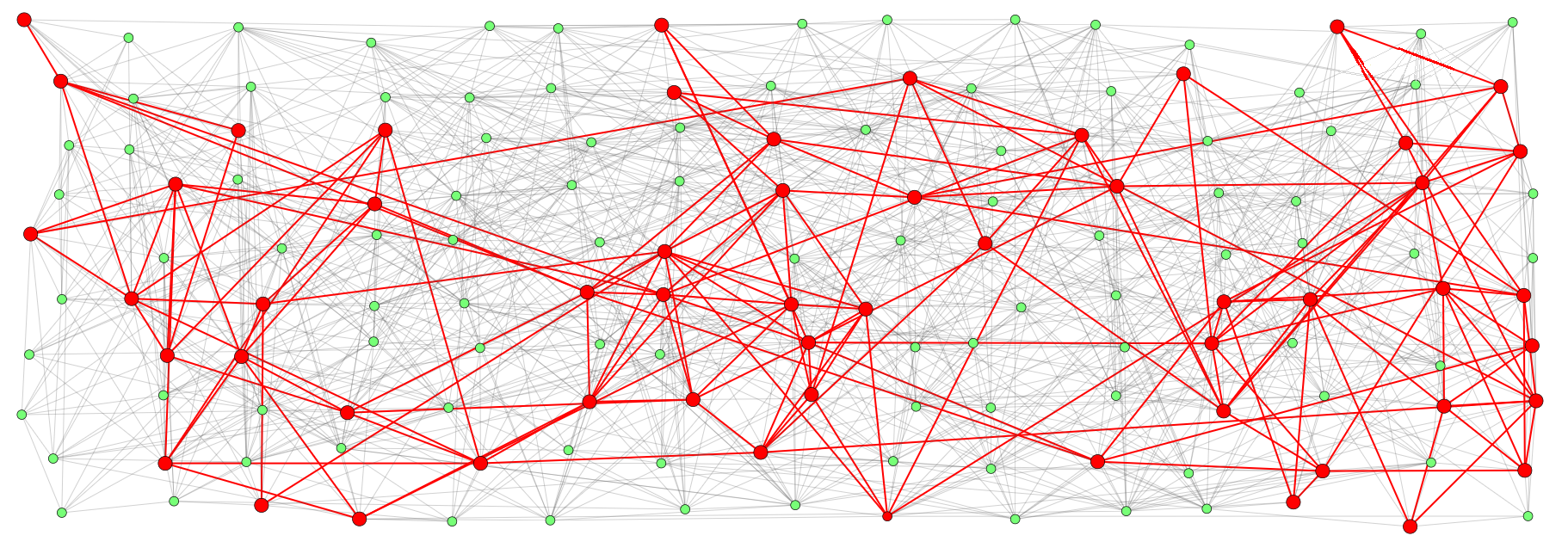
Figure 4: As the probability increases the gossip spreads to a larger part of the network
In summary, arbitrarily removing edges in a graph can yield interesting structures, mathematicians working in percolation theory try to discover these structures for different types of graphs, for example for the complete graph as seen in the example in this article. In percolation theory phase transitions play an important role, which are interesting both mathematically but also in real life.
Did you know that if you divide a pack of cards into 13 piles of 4 cards, then you can always pick one card from each of the 13 piles so that there is exactly one card with each rank? There is some beautiful math behind this puzzle.
If, after reading the title, your immediate response is to shout "1/6-th", then you have correctly answered the question. Well done! However, in this article we will focus on the meaning of this question. What exactly is this "chance" of which you've just exclaimed it equals 1/6-th?
Rafael Prieto-Curiel is a mathematician and a faculty member at the Complexity Science Hub in Vienna, Austria. His research focuses on crime, mobility, migration and urban dynamics. We interviewed Rafael to learn about his story.
 nodes in which the edges between any two neighbors can be open with probability
  (allowing the fluid to pass), or closed with probability
  . In this model, one would like to know how likely it is that an open path (that is, a path, each of which has an "open" connection) from top to bottom.
 grid works. You can choose the probability
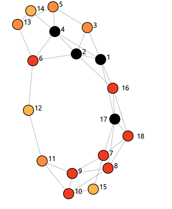
 and
and  .
. , so about half of the edges. This makes sense since every edge is removed with probability 0.5. In Figure 2 we see that 16 edges were removed. If we repeat this experiment several times, we will notice that sometimes more or fewer edges will be removed. This deviation from the expected number of removed edges is described by the variance, which for a binomial distribution is equal to
  , so
, so  in this example.
 nodes and connect all pairs of knots together with one edge. The resulting graph is called in mathematics the complete graph on
  then all edges will definitely be conserved, if
  then all edges will be definitely removed.
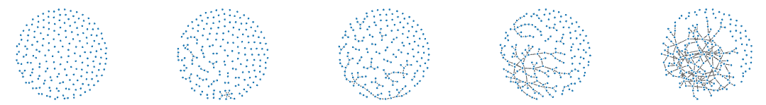
 , and
, and  , with
  , the graph with a high probability is not connected after percolation, but for values of
  , the graph with a high probability is connected! So there is a transition from one phase (not connected) to another phase (connected). The value


 is too low
 comes to know some very catchy gossip. In the next time step, there is a probability
  . We can think of this as the outcome of flipping an unfair coin, which with probability
  ! In the long run, the gossip will spread throughout the entire components containing the first source nodes. When
  , there is a good chance that the first source nodes are in the giant component, with the result that everyone gets to know the gossip!