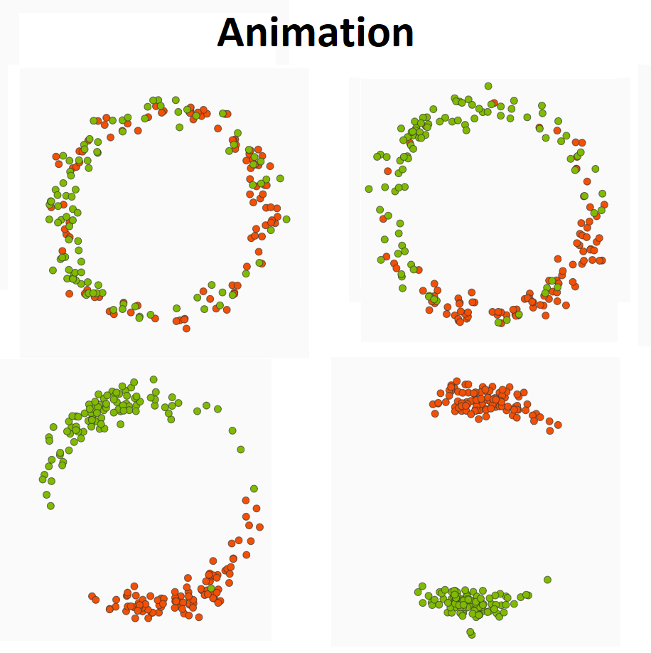
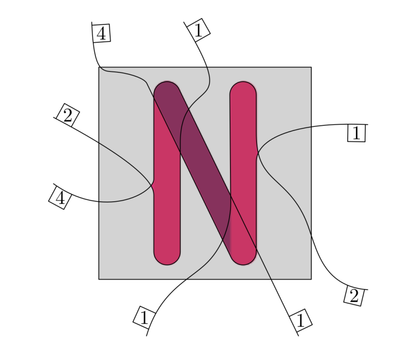
The two community Kuramoto model – Animation

In the interactive simulation below, developed by Martijn Gosgens, you can see how the two-community Kuramoto model works.

In the simulation you are able to adjust a variety of parameters of the model before starting the simulation and seeing what happens. The first parameters you can adjust are the number of nodes (colored dots) in each community. $N_{1}$ represents the number of nodes in the red community and $N_{2}$ the number of nodes in the green community. Next you are able to adjust the strength with which red nodes attract other red nodes ( $K_{1}$ ) and the strength with which green nodes attract other green nodes ( $K_{2}$ ). We are predominantly interested in cases where both $K_{1}$ and $K_{2}$ are positive (but feel free to experiment with negative, i.e. repulsive, $K$ ’s). The parameters $L_{1}$ and $L_{2}$ are the strength with which red nodes are attracted (or repulsed) by green nodes and the strength with which green nodes are attracted by red nodes respectively. When these are positive the interaction between the two communities is attractive, when they are negative the interaction is repulsive. The last model parameter you can adjust is the noise strength, $D$ . This should be greater than or equal to zero and it adjusts the amount that the nodes jiggle. Making $D$ larger makes the nodes jiggle more.

In the next bit of the simulation you can adjust how the dots will be placed on the circle initially (when the simulation starts) as well as the natural properties of the oscillators. With the “Frequencies” option you can select “constant zero” or “standard normal”. Selecting “constant zero” gives each dot the property that it would stand still if there where no other dots and selecting “standard normal” gives each dot its own speed it would rotate around the circle with (drawn from a normal distribution). Finally, you can change how the dots start on the circle. The initial positions are taken randomly from two (normal) distributions. By changing $u_{1}$ and $u_{2}$ you adjust the mean of these distributions and by adjusting the slider for $r_{1}$ and $r_{2}$ you adjust how peaked (concentrated) the distribution is.

Let’s consider an example: We will set the number of nodes to 200 per community. We will set both $K_1$ and $K_2$ to 5, both $L_1$ and $L_2$ to -2 and $D$ to 1. Next we take the Frequencies to be “constant zero”, set both $u$ ’s to 0 and both $r$ ’s to 0.75. This means that the nodes will initially be fairly concentrated (an $r$ of 1 would be that they are all on the same spot, while 0 is completely spread out on the circle) around the zero point on the circle (the right most point on the circle).

Now click on “Restart Simulation” (maybe restart it a couple of times to check if what you see is repeatable). What do you observe? Why? What happens when you change $L_{1}$ to 2 and $L_{2}$ to -3? What do you observe if you choose different values for $r_1, r_2$ ? Take some time to play around with the simulation.

Click here for the answer

What you should see first is that both communities become more concentrated around the zero point. This is as both communities have $K$ ’s of 5 which means the nodes would like to be closer to each other. But of course both $L$ ’s are negative which means that the green and red nodes repel one another, so what you should see next is that the two communities move apart until they are on opposite sides of the circle.

Click here to have a look at the mathematics behind this simulation!

Would you like to stay up to date when a new post appears on the Network Pages?

Subscribe to our mailing list

Related articles

What have Donald Trump, an epidemiologist and a rock in common?••

Eigenvalues to the rescue••

Martijn Gösgens as one of the Faces of Science•

How many colors do you need to color a map?••

Picking up 13 different cards from 13 piles (Part 1)•